Mordred

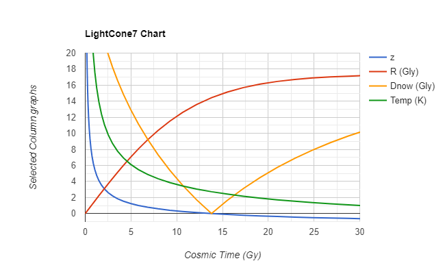
You might want to revisit your dimensional analysis.... You have in the above units units of length on the right hand side of your equations However no corresponding units of length on the left hand side in several of the above such as temperature, power, and luminosity secondly many of the above has non linear rates of change where you have linear. assuming you are dividing the primed value with the unprimed value then you have dimensionless quantities on the LHS. So the RHS definitely does not match in every case in the above. My point 5 is an example of a very distant set of measurements that can be examined using spectrographic evidence. Google Rydberg lines for what that entails. However when you account for redshift the lines show the same distance in the atomic orbitals. No you have not adequately accounted for that as your equations are too linear to handle the nonlinearity of redshift. this is what I am referring to on the nonlinearity note how Z as well as temperature suddenly spikes. Where distance now hits the x axis is the time now... previous to that is the past while to the right is the future using current cosmological parameters. You will also find that the expansion rate ie Hubble parameter is also non linear. In point of detail the above shows logarithmic rates of change. Zero on th x axis corresponds to z= 1100 CMB http://web.mit.edu/2.25/www/pdf/DA_unified.pdf use this and recheck all your equations under proper dimensional analysis

True enough considering all the different variations coordinate time, proper time, conformal time, commoving time. Though in each case it's more accurate to treat these as defined observers.

Unfortunately it does relate in one regard as a common misconception is that a higher density past equates to spacetime curvature and hence time dilation with regards to the FLRW metric. However this isn't the case there is subtle differences in curvature with regards to the FLRW metric to spacetime curvature in GR with regards to time and proper time. Anyways that's likely best left off for a different discussion.

Correct however as I mentioned above you need a cosmological term in combination to the EFE to keep the scale factor constant. Hence Einsteins blunder a static eternal solution is unstable as I mentioned previously

No in the FLRW metric if k=0 then \[T_{\mu\nu}=0\] you still have the scale factor though as that universe can still expand or contract. If the factor is constant at zero you have a static universe which is a special class of solution (Einsteins biggest blunder) and Einstein needed to add a cosmological term to get a= constant zero.

You should reexamine the FLRW metric in particular the ds^2 line element you will find the k=0 metric Euclidean which can be considered space even though the metric includes spacetime with the addition of the scale factor. Besides one of the lessons Minkowskii taught is that you cannot separate space and spacetime.

Regardless of whether your examining space or spacetime isn't doesn't matter in this case a truly flat space or spacetime can still expand or contract when you include radiation or Lambda. You can experiment with this formula which will show this \[H_z=H_o\sqrt{\Omega_m(1+z)^3+\Omega_{rad}(1+z)^4+\Omega_{\Lambda}}\] or use the cosmological calculator in my signature link. It will allow you to set the cosmological parameters

the point is that even if k=0 precisely the universe can still expand due to the kinetic energy terms from radiation and the cosmological constant term. A good way to understand that is to examine the single component toy model universes such as radiation or Lambda only universes alternatively the DeSitter and anti-Desitter universes. It is a good way to examine individual each comp0sition of our universe.

total energy stays constant in the FLRW metric as per an adiabatic (closed system) perfect fluid however the energy density decreases due to expansion and correlates to the cosmological redshift. The common value for number of photons is 10^{90}. That value is calculated via the Bose Einstein statistics for bosons and gives the number density of photons by setting the effective degrees of freedom at 2 for the two polarity states of the photon. For bosons chemical reactions also set to zero. Bose Einstein Statistics (bosons) \[n_i = \frac {g_i} {e^{(\varepsilon_i-\mu)/kT} - 1}\] Fermi-Dirac statistics (fermions) \[ n_i = \frac{g_i}{e^{(\epsilon_i-\mu) / k T} + 1}\] Maxwell Boltzmann (mixed ) \[\frac{N_i}{N} = \frac {g_i} {e^{(\epsilon_i-\mu)/kT}} = \frac{g_i e^{-\epsilon_i/kT}}{Z}\]

That's not quite correct, yes a critically dense universe is homogeneous and isotropic with k=0 precisely. However you can still have expansion if the kinetic energy term exceeds the potential energy term. Our universe is extremely close to flat but not only that it is still considered homogeneous and isotropic. This might surprise you but at inflation the universe was incredibly flat and well as uniform in mass distribution to the order of \[10^{15}\]. One thing to note the critical density applies the mass term with no pressure term by applying matter. The kinetic energy term isn't part of that formula. Neither is the equipment solution in the EFE for a static solution. It is the kinetic energy term that allows for expansion or contraction in a homogeneous and isotropic universe. Such as our universe. A side note tidbit the static solution is what Einstein called his biggest mistake as he attempted to add a different cosmological term to preserve the static solution. He knew the EFE also showed expansion or contraction even with a uniform mass distribution and that a static universe was inherently unstable.

You need to be careful on causal connections. Anything we can see or measure we are causally connected to in essence we are causally connected with our observable universe. I different observer at say 1000 light years away, will have a different observable universe, however would share causal connections where that faraway observers, Observable universe overlaps with ours. Causal connections don't define "now" as we receive signals from the past events. The future can also be causally connected to us from the perspective of a future observer.

Well let's replace gas with plasma. The same plasma used in star formation. Now that plasma is ionized so your dealing with a combination of rotation (conservation of angular momentum). Gravity and the EM field interactions. The EM field isn't involved for DM which is one of the distinctive differences in galaxy formation. When I get home I will find a decent article on how density wave theorem progresses but in essence the flattening into the plane is already underway with the above prior to the majority of star formation. Our galaxy for example has different star ages and also different metalicity percentages. This detail is covered in the density wave theorem.

Hint think of what a Galaxy comprises of prior to BH and stars.

Good answer +1

yes this is precisely the direction I wanted you to take, these equations are ideally suited. Good find key note on equation 5.5.4 in regards to specific acoustic impedance involving a linear, lossless wave equation.

I would highly recommend you look into independence in particular for planar and spherical waves. You should also be able to match up to the relevant logarithmic functions as they apply to acoustics. If your not it indicative of an error or some missed factor. Once you get into more than one wave you will definitely need to factor in your wave equations primarily in amplitude and phase angles. In essence constructive and destructive interference factors.

let me guess your adding two waves of opposite phase and seeing c_o disappear ? still going through your math but I'm glad to see you got the displacement phase lag that showed in the reference I posted though the graph in the article isn't very clear. here is a decent article to use for comparision https://hal.archives-ouvertes.fr/hal-03188302/document

That just leads to a whole range of misconceptions. It's better and more accurate to simply point out that anything moving at c isn't an inertial frame of reference. Hence follows a null geodesic.

Lmao now there's an expression to deflate one's ego lmao

I like your example it also does an excellent job of showing degrees of freedom with the rotations etc. +1

A dimension is a mathematical term for a degree of freedom or some indepenendent variable. The spatial dimensions x,y,z can each vary without the other variables varying. Time we give dimension of length by the interval (ct) the distance light travels in one second.

In essence yes though the methods vary. I can't recall the theorem name but any infinite set has a finite portion. All gauge groups are finite

No its actually very easy think of a graph. Now set the max value at 1 (max value for a normalized unit. Now take the bell curve as it trends to 0 and 1 on that graph. Lets use the infrared end, divide 1 by a 1/2 with each result being further divided by 1/2 until you reach 0. You will never reach 0 that is an example of diverging to infinity. You have an infinite number of 1/2 divisions. So you apply some cutoff. (reqularization

In math language normalized units such as c=h=k=g=1. If you have a field such as the EM field you have the normalization via the quanta given Planck units. That's included in the previous expression. Divergence means diverges to infinity where you typically have two points on a graph that this applies. \[0\leftarrow x \rightarrow\infty\] QFT has a regulator to provide an effective cutoff before those two points apply. The infrared regulator and the ultraviolet regulator. these will vary depending on the theory. The more common is dimensional regularization.

That would still be accurate as a quantum theory would have to be divergence free. In essence normalized. QFT for example has the infrared and ultraviolet cutoffs for the \[SU(3)\otimes SU(2)\otimes U(1)\] gauges of the SM model.