Why are mathematicians afraid of contradictions? In my opinion, contradictions should be afraid of physics, and mathematicians study everything that can be imagined. So why not head into the world of prohibitions and experiment with "absolute mathematical completeness"? In this article, I will briefly try to describe the results of my observations. Here you will not see the hard evidence on which my assumptions are based. All the same, they will not be interesting to anyone. I just want to get people interested in looking for new ways to code. Binary classical and quantum systems are not the only ways of ordering information, and for some reason no one talks about this, and does not attempt to find other, larger-scale options. The geometrical interpretation of information theory, recently considered here, is the origin of such a view, but it boils down to the probability of the occurrence of events under conditions of entropy.
Take a look at my artistic version of full diversity, which I sometimes tell my little brother instead of a bedtime story.
A bonus awaits you at the end. I will show you how you can encode the volume of normal air !!! To do this, you only need a cylinder and a piston, which, with the help of the correct combination of back-and-forth movements, generates a full-fledged, self-sufficient algorithm. The structure of this algorithm is not only particles, but also the voids between them.
For some systems, I had to give my own names, which may scare you away, but take this as a child's fantasy. It is not my fault that these systems are still not open. No work is being done in this direction due to internal contradictions between the unification of higher order logics. But, can you prove that it is impossible to identify a consistent system from a contradictory system? I doubt it.
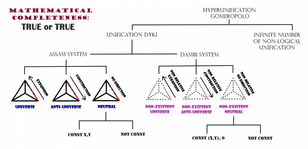
Mathematical completeness (Everything that exists)picture1. Mathematical completeness (Everything that exists)
Assam's system is a second-order logic, an integral part of a higher-order logic, the Dyki unification. It consists of two types of vectors. Constantly tapering and expanding. In the Assam system, three (four, taking into account two neutrals) are possible relative types of motion, carried out by the method of shifting vectors from one area to another. The displacements are a consequence of the compression of the red vectors and the stretching of the blue vectors indicated in Figure 1. The arrows indicate the general direction of motion of the array of some combination.
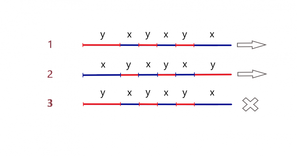
picture2. Types of movements.
Neutral, between the first and second types of variability. As in the non-existent world of the Dambi system, in the neutral there is no interaction, of any internal system with the external one. Because there is no relativity, and, therefore, there is no time, mass, speed, temperature and other calculated values arising from the impossibility of comparing something, analyzing one local variability relative to another, due to the lack of such internal operations as integration and differentiation between maternity and continuous values. The neutral, in turn, is subdivided into two levels of constant dependence. More on this below. The variety of the third case can only be obtained from the first and second. The displacements in the first two cases are carried out in the full range from a single shift of the minimum value to a specific array of the maximum value. The sequence of shifts is strictly relative. The more often the values x and y alternate on a given scale (segment), the faster the changes will take place there, because regardless of size, each vector moves in both directions at the same infinite speed.
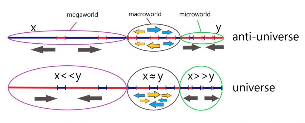
In the universe, an increasing rate of change can be observed at the atomic level of the microcosm, and at the intergalactic level of the megaworld. This happens within the framework of quantum mechanics, and for a number of other "mysterious" reasons associated with dark energy, dark matter, and God knows what else is dark. When physicists do not understand something, they begin to invent phenomena with the "dark" prefix. The main factor is the vantage point.
Let's imagine all the possible options for alternating rows of continuously converging and diverging, which personify vacuum and pressure, respectively.
picture3.Neutral "no const"
picture4.Neutral "x,y = const"
picture5.Anti-universe and universe
What constants are, why are they needed and where do they come from.
For the Assam system, the following set of constants is valid:
Antiuniverse: y = const = 1, → ∞ x > ∞ y;
Universe: x = const = 1, → ∞ x < ∞ y;
Neutral1: x, y = const (0; ∞), → ∞ x = ∞ y;
Neutral2: not const, → ∞ x = ∞ y.
Constants are fixed values. These are the reference points for pinpointing local contraction or expansion. They determine the approach to zero or infinity. Thanks to the constants (and their absence in the fourth case), Assam's system can be divided into four types of movements.
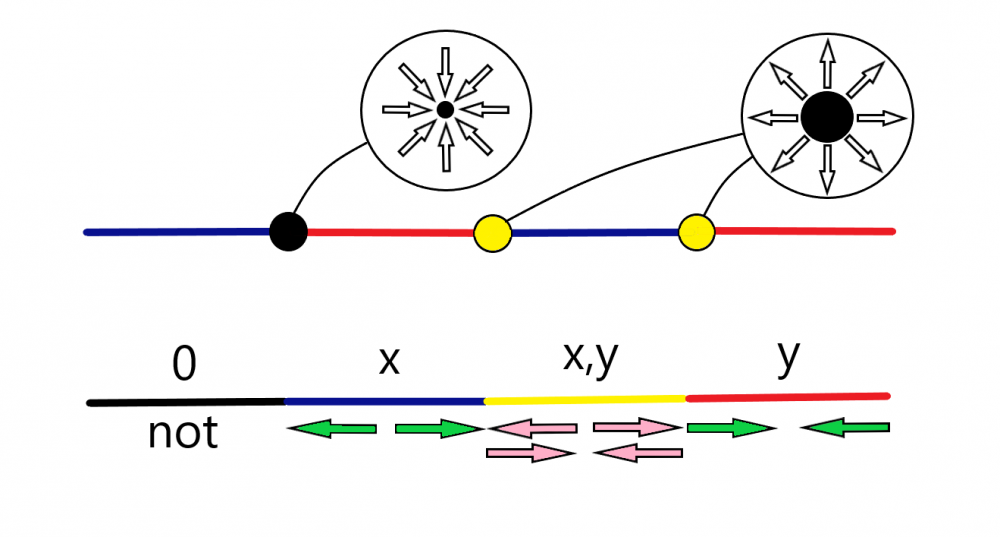
picture6.Four types of minimum values (vectors), existing and non-existent representations of geometric variability and non-variability. Possible combinations of infinity.
The figure shows the Assam system (x + y), together with the Dumby system (x, y + 0). The depicted two straight lines from compound colored lines, which can be extended indefinitely, and combined with each other in a complete enumeration 2 ^ x. If, in the case of an infinite increase at any point x, there can be y, then x = y. Accordingly, in the general Assam system, the pressure is equal to vacuum. They differ only on a specific, relative scale.
Conditions under which the value of y grows into the value of x:
picture7.∞x = ∞y
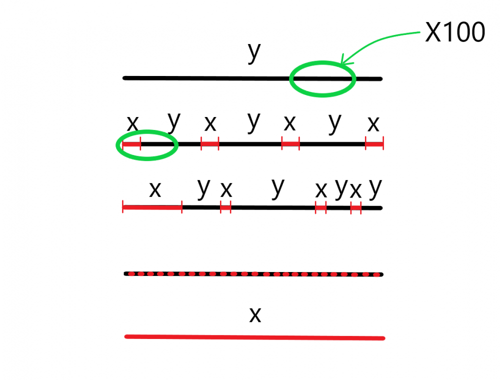
Let us choose an arbitrary section on a continuous continuously narrowing vector y (emptying) and increase it many times, for example, by a factor of 100. Then the points x will emerge that were not there before. At large scales, they were ignored by the system. A limited computing system cannot perceive values less than its own minimum value, relative scale. After repeating the enlargement operation, new, smaller X's appear on the second line from the top. Moreover, they can be in various places, but the important condition is that all black lines should always be longer than red ones. It turns out to be a funny situation. The red vector of expansion can be located at any infinitesimal point of the black vector of contraction, which means that in a non-relative system, it is it. However, even in a non-relative system, the common vector will narrow at all infinitesimal points.
If, y is not taken into account, then the site will turn into a full-fledged infinite extension of x. And, the most interesting thing is that not one vector is not initially determined by the properties of compression or expansion. This means that not one infinity clearly prevails over the other. The original red expansion vector may be a black contraction vector, the prevailing values of which are lost at infinitely rapidly changing scales. And vice versa. This may seem inconceivable. It turns out that any converging series is divergent, under conditions of infinitely fast approximation. One and the same infinity can become larger, or it can become smaller, relative to another infinity.
The mere formulation of such an assumption, in its complexity, can surpass all the "Millennium Prize Challenges" in the field of mathematics.
Take, an arbitrary vector y, which is the minimum value of some system. The range of x, y ratios inside it will look like this:
if x = 0.0∞1, then y = 0.9∞9,
if x = 0.49∞9, then y = 0.50∞1
I do not want to dwell on the Dumby system for a long time. Let us take into account only the fact that, like the Assam system, there are two opposite types of variability. An infinitely large point is obviously also infinitely small, as it contains an infinite number of small points, and vice versa, at each infinitely small point, there is a set of infinitely large ones. The minimum values of the Dambi system are isolated from each other and cannot be calculated using the Assam system. It is a non-relative view, with the opposite computational process of variability. During this process, changes do not occur. In this case, it is impossible to accept the influence of the external system to the internal system until the internal system itself embraces the external one.
The logical union of Dyki is the basic logic of a higher order, which is built on eighteen dimensions, with a minimal, tetrahedral form. Of the myriad of other non-logical associations of Homeopolo, with minimal forms, based on dimensions, from zero to infinity. Homeopolo is a "super-highest order" logic. It cannot be calculated, not by one other system of unions, since it has infinite types of infinities, respectively, and an infinite difference between them. However, in its absolute completeness, Homeopolo can calculate itself, which means that it does not contradict the law of perfect mathematical versatility, on which the postulate of general representations of this concept is based. Dyki is a special case.
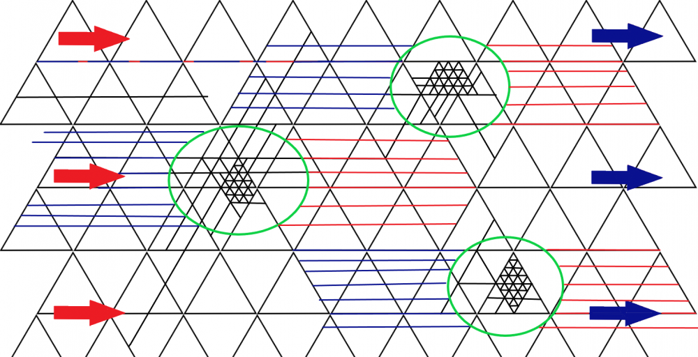
Setting the speed of directional movement is carried out by entering ⸎ and three conditional cycles. To move arrays of a certain scale in a given direction, you must set the following conditions:
In front of the vector place the cycle y = const, and behind the array, place the cycle x = const. The array itself has all three cycles, as it is an equilibrium zone.
picture8.
Vector mesh. Unbalancing the array.
At y = const = 1, → ∞ x > ∞ y - the common section expands;
When x = const = 1, → ∞ x < ∞ y - the common section is narrowed;
For x, y = const (0; ∞), → ∞ x = ∞ y - the common section does not change;
At not const or x = n, y = n, → ∞ x = ∞ y - the common section does not change.
Let's designate the zone of the array. It will be an arbitrary vector, the "Gladon frame".
Begin:
In order to keep the algorithms of the given sequences, a continuous cycle of transformation of x pressure into y discharge is needed and vice versa.
picture9.
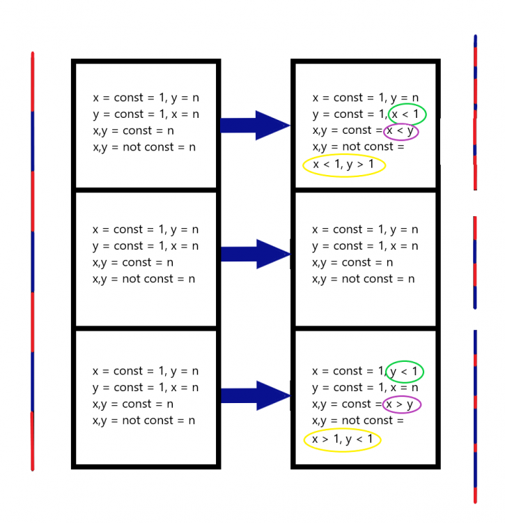
Algorithm transformation on the example of a three-sector vector. Move up for the middle section.
From this figure, you can see exactly how the system looks in equilibrium (left), and what changes need to be made in order, for example, to move upward (right). When entering the program of holding algorithms, the array of the lower section will begin to create continuous pressure, predominantly by the dimension x. An array of the upper section, having a continuous discharge, usually having y. In the middle section, the array remains unchanged. It is assumed that this area, or rather what is in it, will move upward, but the partitions should not be insulating.
Code outline:
For the first section (vacuum):
Begin:
x = const = 1, y > 1;
y = const = 1, x < 1;
x, y = const = x < y;
x, y = not const = x < 1, y > 1;
t0 = (x / n + y / n) * n = 0;
t1 = (x / n + y / n) * n = 1;
t0 + t1 = const x, const y = 1;
n (1; ∞) is the dimension of x, y;
N (1; ∞) is the number by which the sum of x or y is divisible.
Decision:
if x = const >, < 1; y <, = 1 then
y n = t0 = (sum 0 < y n <0.5) + (sum 0.5 < x n < 1) = 1,
y n = t1 = (sum 0.5 < x n <1) / N = (sum 0 < y n < 0.5) = 1,
if t0 + t1 > 1, then (x / n + y / n) * n + +
if t0 + t1 < 1, then (x / n + y / n) * n - -
if y = const>, <1; x>, = 1 then
y n = t0 = (sum 0 < y n < 0.5) + (sum 0.5 < x n < 1) = 1,
y n = t1 = (sum 0.5 <x n <1) / N = (sum 0 < y n < 0.5) = 1,
if t0 + t1> 1, then (x / n + y / n) * n + +
if t0 + t1 <1, then (x / n + y / n) * n - -
if x, y = const = x >, = y then
x, y = const, x n = y n, then x = 0, y = 0; and if x, y = const = x n > y n,
y n = t0 = (sum 0 < y n < 0.5) + (sum 0.5 < x n < 1),
y n = t1 = (sum 0.5 < x n < 1) / N = (sum 0 < y n < 0.5) = 1,
if t0 + t1 > 1, then (x / n + y / n) * n + +
if t0 + t1 < 1, then (x / n + y / n) * n - -
if x, y = not const = x >, = 1; y <, = 1 then
x, y = not const, x n = y n, then x = 0, y = 0; and if x, y = const = x n> 1, y n <1,
y n = t0 = (sum 0 < y n < 0.5) + (sum 0.5 <x n <1),
y n = t1 = (sum 0.5 < x n < 1) / N = (sum 0 < y n < 0.5) = 1,
if t0 + t1 > 1, then (x / n + y / n) * n + +
if t0 + t1 < 1, then (x / n + y / n) * n - -
For the second section (pressure):
Begin:
x = const = 1, y < 1;
y = const = 1, x > 1;
x, y = const = x > y;
x, y = not const = x > 1, y < 1;
t0 = (x / n + y / n) * n = 0;
t1 = (x / n + y / n) * n = 1;
t0 + t1 = const x, const y = 1;
Decision:
if x = const >, < 1; y >, = 1 then
x n = t0 = (sum 0 < x n < 0.5) + (sum 0.5 < y n < 1) = 1,
x n = t1 = (sum 0.5 < y n < 1) / N = (sum 0 < x n < 0.5) = 1,
if t0 + t1 > 1, then (x / n + y / n) * n + +
if t0 + t1 < 1, then (x / n + y / n) * n - -
if y = const>, <1; x <, = 1 then
x n = t0 = (sum 0 < x n < 0.5) + (sum 0.5 < y n < 1) = 1,
x n = t1 = (sum 0.5 < y n <1) / N = (sum 0 < x n < 0.5) = 1,
if t0 + t1 > 1, then (x / n + y / n) * n + +
if t0 + t1 < 1, then (x / n + y / n) * n - -
if x, y = const = x <, = y then
x, y = const, x n = y n, then x = 0, y = 0; and if x, y = const = x n <y n,
x n = t0 = (sum 0 < x n < 0.5) + (sum 0.5 < y n < 1) = 1,
x n = t1 = (sum 0.5 < y n < 1) / N = (sum 0 < x n < 0.5) = 1,
if t0 + t1 > 1, then (x / n + y / n) * n + +
if t0 + t1 < 1, then (x / n + y / n) * n - -
if x, y = not const = x <, = 1; y>, = 1 then
x, y = not const, x n = y n, then x = 0, y = 0; and if x, y = not const = x n> 1, y n <1,
x n = t0 = (sum 0 < x n < 0.5) + (sum 0.5 < y n < 1) = 1,
x n = t1 = (sum 0.5 < y n < 1) / N = (sum 0 < x n < 0.5) = 1,
if t0 + t1 > 1, then (x / n + y / n) * n + +
if t0 + t1 < 1, then (x / n + y / n) * n - -
Implementation:
picture10.
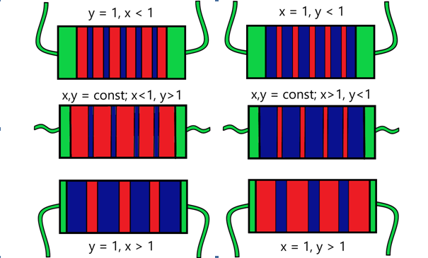
The simplest example of creating a one-dimensional environment for coding by the "pulsating membrane" method.
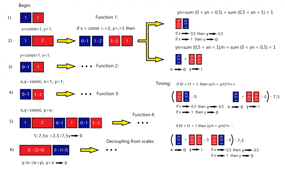
In order to capture all the states of the source, compiling, and final code, conditions must be created to simulate such relative positions. The figure clearly demonstrates the fixation of all cases of sequences (except for x> y, and y> x, which combine the three above cases). Having placed atmospheric pressure in a cylindrical vessel, it is also necessary to place in them movable membranes (pistons) indicated in green, under the control of a microcontroller. In this case, atmospheric pressure, or simply air, will be the object of coding, and the pistons, with the help of backward translational movements, impulses assigned to them, cyclic conditions, are coding tools. The principle of this coding is somewhat similar to the coding of CNC machines. The only difference is that the initial, conditional operations, contributing to the binding of air to the necessary conditions and cycles, are carried out mechanically in a standard way (using signals from an electronic microcontroller). But, when the program is ready, the cause-and-effect relationships must independently continue to generate a cyclic compilation, from eight conditions and eight decisions, based on replacing the variables x and y with each other locally and in full. The whole difficulty lies in the injection of the code. It is necessary to force unmanaged algorithms to respond to the commands given to them. How can this be done? We know that in a neutral environment, taken as a relative reference point, or zero point, there are all possible algorithms. The following actions are such that from logical completeness, it is necessary to single out several special cases. And, to do this in such a way as not to ignore the wrong (unnecessary) sequences, but to rebuild them into the necessary ones using the previously considered cycles that simulate decoupling from scales and relativity. Having set the timings, to 1, in non-relative local loops, we set them the execution time, for the fastest relative value.
picture11.
Vacuum zone coding algorithm.
The numbers in the figure indicate the amount of air injection (in blue squares) and air evacuation (in red), in cm ^ 3. To obtain a valid algorithm, you must strictly follow the sequence of actions. Even when writing these values, it is important to write constants in the first step so that in the fourth step, when a floating value y (1-2) is received, start from one, and not from zero, as in the previous cases. The first action is needed in order to borrow 1y from there, x is not needed, it is written just like that, there is no need for it. The first step is to create a backup data store. The sixth action, for example, requires an initial y - 4, but it is taken from 2,3,4 actions, so there is no need to create additional reserves. The fifth action is the sum of 2,3,4 actions. Actions of the 0-1 format take place directly at the moment of movement. That is, if 0-1 is specified, this is an infinite number of values in this interval. To obtain such an effect, it is necessary to reduce the volume of the cylinder (when dividing), without affecting at all the density, pressure / vacuum values. When, for example, the selected area tends to zero, it must maintain the overall ratio of x and y densities.
The first function, arising from the contradictions of the first condition, directs the algorithm to correct it, rebuild or “cyclical balancing”. If the initial conditions are not met, then, in the minimum value, const = 1, x prevails over y. Let's equate x to y so that y occupies most of the const, and tends to 1. For this, the funniest fraud is performed, catching y (0-0.5) on all x (0.5-1). After that, it remains to set the time to create a fixed time for performing cyclic balancing. Bind the initial time to 0, and the final time to the minimum const value. If the time conditions are not met, due to the low speed, then the alternation throughout the volume increases, in the direction of cyclical balancing, thus accelerating the rate of variability. If, on the contrary, it is necessary to slow down the speed, as indicated in the lower right corner, the increase in the alternations is carried out in the direction of unbalance. Also, the time depends on the number of algorithms in the volume of the cylinder, which are set separately. Similar to the first function, the other 3 functions are generated. The sixth action completely decouples from the scale, and only after it can functions be built on any site.
Do you understand anything? Ask questions.

